It is very hard to determine if any asset or really anything whose value is represented by a series of prices is cheap or expensive. This is a tool that incorporates technical analysis tools in order to determine whether prices have been extended to the upside or to the downside in relative terms, given the history of a certain asset.
Moving Averages
A moving average is a calculation that takes the arithmetic mean of a given set of prices over a specific number of periods in the past. This indicator is the main building block of this Risk Metric tool.
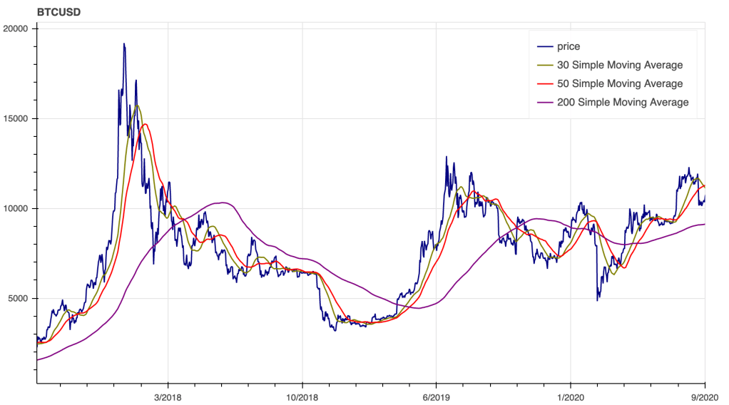
Above we display 3 simple moving averages for the same time series of BTC prices for 30, 50 and 200 days respectively. Moving averages of shorter duration follow up the price more closely, while longer duration moving averages move slowly. What will particularly interest us is the interaction between different moving averages, specifically the ratio between them. Let us examine this idea.
Consider the abstract ratio: shorter moving average / longer moving average.
How would that ratio behave in different situations? Well, the bigger the ratio, the more difference there is between the shorter and longer moving average, specifically the shorter moving average in this case is bigger than the longer one, indicating an uptrend. The bigger the difference between them, the more overextended the price becomes. The opposite holds for the downside extension of prices.
While there is no absolute limit as to how big or small the ratio can become, it can be proven to be a quite valuable statistic as we can mark the value of the ratio in historical peaks and troughs and get a “sense” as to how overextended the price is, given historical data. In fact we can use this metric to judge overextension across different assets because the ratio nullifies the difference of price scales between them. That is to say, if we now in the energy sector 10 relevant stocks had peaks where the ratio had values between, say 2.2 and 2.5, we can assume that similar stocks might behave the same. Therefore we can better identify great entry and exit points for out investments in these stocks.
Now, what values should the moving averages have? Well that is up to trial and error and maybe some optimisation. For starters, it would be nice to reference many short/long moving average ratios in order to average out any overfitting that might occur by only choosing 2 specific values. We can then normalise each individual ratio and then take the average of their sum.
Let  be a set of moving averages in ascending order. To construct the set of ratios between pairs we need to consider all the possible combinations of the type
  moving average.
For example, if we had 4 moving averages
moving average.
For example, if we had 4 moving averages  the exhaustive combination of ratios would be
  or
or  It is not necessary to get the exhaustive combination of all possible pairs. We might decide that moving averages closer to each other are not that informative about price movements(usually the case). It is up to individual use case for us to determine which pairs would accomplish our goals.
Let
It is not necessary to get the exhaustive combination of all possible pairs. We might decide that moving averages closer to each other are not that informative about price movements(usually the case). It is up to individual use case for us to determine which pairs would accomplish our goals.
Let  be the set of ratios we come up with. We are going to normalise them and sum them like so.
Here we normalise the ratios(to the interval [0,1]) so we can sum up similar quantities. There is a case to be made for summing up the ratios as is and establishing a different range for out Risk Metric.
be the set of ratios we come up with. We are going to normalise them and sum them like so.
Here we normalise the ratios(to the interval [0,1]) so we can sum up similar quantities. There is a case to be made for summing up the ratios as is and establishing a different range for out Risk Metric.
 Now we have the base formula for our Metric. In the iteration below I have chosen to blend this metric with the RSI(Relative Strength Index) indicator for more robust results. So my version of the formula becomes
 where
where  and for this case
For this example we can draw numbers from the Fibonacci sequence that will represent
import pandas as pd
import numpy as np

class RiskMetricNormalized:

    def __init__(self, dataset, price_col,  date_col, ema_periods, rsi_periods):
        self.dataset = dataset
        self.price_col = price_col
        self.date_col = date_col
        self.ema_periods = sorted( ema_periods )
        self.rsi_periods = rsi_periods
        self.data = self.RSI_composite()
        self.pairs_list = self.ema_pairs()
        self.data_ema_risk = self.ema_risk(self.data)
        self.df = self.total_risk()


    @staticmethod
    def NormalizeData(data):
        return (data - np.min(data)) / (np.max(data) - np.min(data))


    @staticmethod
    def Fibonacci(n):

        if n<=0:
            print("Incorrect input")
        # First Fibonacci number is 0
        elif n==1:
            return 0
        # Second Fibonacci number is 1
        elif n==2:
            return 1
        else:
            return Fibonacci(n-1)+Fibonacci(n-2)


    @staticmethod
    def RSI(df, n = 14):

        df['change'] = df['close'].diff(1) # Calculate change
        # calculate gain / loss from every change
        df['gain'] = np.select([df['change']>0, df['change'].isna()],
                            [df['change'], np.nan],
                            default=0)
        df['loss'] = np.select([df['change']<0, df['change'].isna()],
                            [-df['change'], np.nan],
                            default=0)

        # create avg_gain /  avg_loss columns with all nan
        df['avg_gain'] = np.nan
        df['avg_loss'] = np.nan

        # keep first occurrence of rolling mean
        df['avg_gain'][n] = df['gain'].rolling(window=n).mean().dropna().iloc[0]
        df['avg_loss'][n] = df['loss'].rolling(window=n).mean().dropna().iloc[0]

        # Alternatively
        '''
        df['avg_gain'][n] = df.loc[:n, 'gain'].mean()
        df['avg_loss'][n] = df.loc[:n, 'loss'].mean()
        '''
        # This is not a pandas way, looping through the pandas series, but it does what you need
        for i in range(n+1, df.shape[0]):
            df['avg_gain'].iloc[i] = (df['avg_gain'].iloc[i-1] * (n - 1) + df['gain'].iloc[i]) / n
            df['avg_loss'].iloc[i] = (df['avg_loss'].iloc[i-1] * (n - 1) + df['loss'].iloc[i]) / n

        # calculate rs and rsi
        df['rs'] = df['avg_gain'] / df['avg_loss']
        df['rsi'+'_'+str(n)] = ( 100 - (100 / (1 + df['rs'] )) ) /100
        df = df.drop( columns = ['rs','avg_gain', 'avg_loss', 'change', 'gain', 'loss' ] )

        return df


    def RSI_composite(self):

        periods = self.rsi_periods.copy()
        df = self.dataset.copy()

        for p in periods:
            if len(df) > p:
                df = self.RSI(df, p)
            else:
                continue

        rsi_cols = [col for col in df.columns if 'rsi' in col]

        df['rsi_composite'] = df[rsi_cols].sum(axis=1) / len( rsi_cols )
        #normalize
        df['rsi_composite'] = RiskMetricNormalized.NormalizeData(
            [el for el in df['rsi_composite'].to_list()]
        )
        df.replace(0, np.nan, inplace = True)

        return df


    def ema_pairs(self):

        emas  = self.ema_periods.copy()

        ratios = []

        for i in range(len(emas)):

            tmp_list = emas[i:]

            for j in range(len(tmp_list)):
                if j<=1: #because we want ratios of numbers that are at least 2 places apart when ordered
                    continue
                else:
                    ratios.append( [ tmp_list[0], tmp_list[j] ] )

        return ratios


    def ema_ratio(self, df, periods):

        #shorter ema / longer ema

        ema_short = periods[0]
        ema_long = periods[1]

        ema_short_name = 'ema' + str(ema_short)
        ema_long_name = 'ema' + str(ema_long)

        ema_short_name = df[ self.price_col ].ewm(span = ema_short).mean().values
        ema_long_name = df[ self.price_col ].ewm(span = ema_long).mean().values

        ratio = []
        for i,j in zip(ema_short_name, ema_long_name):
            ratio.append( i / j )

        normalized_ratio = RiskMetricNormalized.NormalizeData(ratio)

        df['ema_ratio' + str(ema_short) + '_' + str(ema_long)] = normalized_ratio

        return df


    def ema_risk(self, df):

        ema_pairs = self.pairs_list.copy()

        for pair in ema_pairs:
            df  = self.ema_ratio(df, pair)

        cols_to_sum = [col for col in df if 'ema_ratio' in col]

        df['ema_risk'] = df[cols_to_sum].sum(axis=1) / len( cols_to_sum )

        #normalize
        df['ema_risk'] = RiskMetricNormalized.NormalizeData(
            [el for el in df['ema_risk'].to_list()]
        )
        return df


    def total_risk(self):

        df = self.data

        df['total_risk'] = df[['ema_risk', 'rsi_composite']].sum(axis=1) / 2

        #normalize
        df['total_risk'] = RiskMetricNormalized.NormalizeData(
            [el for el in df['total_risk'].to_list()]
        )

        return df[['total_risk', self.date_col, self.price_col,
                    'ema_risk', 'rsi_composite']]
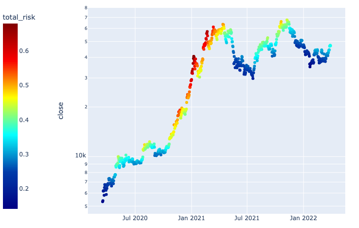
A color-coded example of the results this metric can produce.